5 Data Manipulation with dplyr
https://learn.datacamp.com/courses/data-manipulation-with-dplyr
Main functions and concepts covered in this BP chapter:
select()arrange()desc()filter()mutate()count()group_by()summarize()ungroup()slice_min()slice_max()starts_wth()ends_with()rename()relocate()%in%lag()
Packages used in this chapter:
## Load all packages used in this chapter
library(tidyverse) #includes dplyr, ggplot2, and other common packages
## ── Attaching core tidyverse packages ──────────────────────── tidyverse 2.0.0 ──
## ✔ dplyr 1.1.4 ✔ readr 2.1.6
## ✔ forcats 1.0.1 ✔ stringr 1.6.0
## ✔ ggplot2 4.0.1 ✔ tibble 3.3.0
## ✔ lubridate 1.9.4 ✔ tidyr 1.3.1
## ✔ purrr 1.2.0
## ── Conflicts ────────────────────────────────────────── tidyverse_conflicts() ──
## ✖ dplyr::filter() masks stats::filter()
## ✖ dplyr::lag() masks stats::lag()
## ℹ Use the conflicted package (<http://conflicted.r-lib.org/>) to force all conflicts to become errorsDatasets used in this chapter:
## Load datasets used in this chapter
counties <- read_rds("data/counties.rds")
babynames <- read_rds("data/babynames.rds")
Tip: don’t forget the pipe (%>%) between each step
5.1 Transforming Data with dplyr
Let’s first observe the data we will be working with.
## Rows: 3,138
## Columns: 40
## $ census_id          <chr> "1001", "1003", "1005", "1007", "1009", "1011", "10…
## $ state              <chr> "Alabama", "Alabama", "Alabama", "Alabama", "Alabam…
## $ county             <chr> "Autauga", "Baldwin", "Barbour", "Bibb", "Blount", …
## $ region             <chr> "South", "South", "South", "South", "South", "South…
## $ metro              <chr> "Metro", "Metro", "Nonmetro", "Metro", "Metro", "No…
## $ population         <dbl> 55221, 195121, 26932, 22604, 57710, 10678, 20354, 1…
## $ men                <dbl> 26745, 95314, 14497, 12073, 28512, 5660, 9502, 5627…
## $ women              <dbl> 28476, 99807, 12435, 10531, 29198, 5018, 10852, 603…
## $ hispanic           <dbl> 2.6, 4.5, 4.6, 2.2, 8.6, 4.4, 1.2, 3.5, 0.4, 1.5, 7…
## $ white              <dbl> 75.8, 83.1, 46.2, 74.5, 87.9, 22.2, 53.3, 73.0, 57.…
## $ black              <dbl> 18.5, 9.5, 46.7, 21.4, 1.5, 70.7, 43.8, 20.3, 40.3,…
## $ native             <dbl> 0.4, 0.6, 0.2, 0.4, 0.3, 1.2, 0.1, 0.2, 0.2, 0.6, 0…
## $ asian              <dbl> 1.0, 0.7, 0.4, 0.1, 0.1, 0.2, 0.4, 0.9, 0.8, 0.3, 0…
## $ pacific            <dbl> 0.0, 0.0, 0.0, 0.0, 0.0, 0.0, 0.0, 0.0, 0.0, 0.0, 0…
## $ citizens           <dbl> 40725, 147695, 20714, 17495, 42345, 8057, 15581, 88…
## $ income             <dbl> 51281, 50254, 32964, 38678, 45813, 31938, 32229, 41…
## $ income_err         <dbl> 2391, 1263, 2973, 3995, 3141, 5884, 1793, 925, 2949…
## $ income_per_cap     <dbl> 24974, 27317, 16824, 18431, 20532, 17580, 18390, 21…
## $ income_per_cap_err <dbl> 1080, 711, 798, 1618, 708, 2055, 714, 489, 1366, 15…
## $ poverty            <dbl> 12.9, 13.4, 26.7, 16.8, 16.7, 24.6, 25.4, 20.5, 21.…
## $ child_poverty      <dbl> 18.6, 19.2, 45.3, 27.9, 27.2, 38.4, 39.2, 31.6, 37.…
## $ professional       <dbl> 33.2, 33.1, 26.8, 21.5, 28.5, 18.8, 27.5, 27.3, 23.…
## $ service            <dbl> 17.0, 17.7, 16.1, 17.9, 14.1, 15.0, 16.6, 17.7, 14.…
## $ office             <dbl> 24.2, 27.1, 23.1, 17.8, 23.9, 19.7, 21.9, 24.2, 26.…
## $ construction       <dbl> 8.6, 10.8, 10.8, 19.0, 13.5, 20.1, 10.3, 10.5, 11.5…
## $ production         <dbl> 17.1, 11.2, 23.1, 23.7, 19.9, 26.4, 23.7, 20.4, 24.…
## $ drive              <dbl> 87.5, 84.7, 83.8, 83.2, 84.9, 74.9, 84.5, 85.3, 85.…
## $ carpool            <dbl> 8.8, 8.8, 10.9, 13.5, 11.2, 14.9, 12.4, 9.4, 11.9, …
## $ transit            <dbl> 0.1, 0.1, 0.4, 0.5, 0.4, 0.7, 0.0, 0.2, 0.2, 0.2, 0…
## $ walk               <dbl> 0.5, 1.0, 1.8, 0.6, 0.9, 5.0, 0.8, 1.2, 0.3, 0.6, 1…
## $ other_transp       <dbl> 1.3, 1.4, 1.5, 1.5, 0.4, 1.7, 0.6, 1.2, 0.4, 0.7, 1…
## $ work_at_home       <dbl> 1.8, 3.9, 1.6, 0.7, 2.3, 2.8, 1.7, 2.7, 2.1, 2.5, 1…
## $ mean_commute       <dbl> 26.5, 26.4, 24.1, 28.8, 34.9, 27.5, 24.6, 24.1, 25.…
## $ employed           <dbl> 23986, 85953, 8597, 8294, 22189, 3865, 7813, 47401,…
## $ private_work       <dbl> 73.6, 81.5, 71.8, 76.8, 82.0, 79.5, 77.4, 74.1, 85.…
## $ public_work        <dbl> 20.9, 12.3, 20.8, 16.1, 13.5, 15.1, 16.2, 20.8, 12.…
## $ self_employed      <dbl> 5.5, 5.8, 7.3, 6.7, 4.2, 5.4, 6.2, 5.0, 2.8, 7.9, 4…
## $ family_work        <dbl> 0.0, 0.4, 0.1, 0.4, 0.4, 0.0, 0.2, 0.1, 0.0, 0.5, 0…
## $ unemployment       <dbl> 7.6, 7.5, 17.6, 8.3, 7.7, 18.0, 10.9, 12.3, 8.9, 7.…
## $ land_area          <dbl> 594.44, 1589.78, 884.88, 622.58, 644.78, 622.81, 77…
5.1.1 Select
This allows you to choose which variables/columns to include from a dataset.
## # A tibble: 3,138 × 4
##    state   county   population poverty
##    <chr>   <chr>         <dbl>   <dbl>
##  1 Alabama Autauga       55221    12.9
##  2 Alabama Baldwin      195121    13.4
##  3 Alabama Barbour       26932    26.7
##  4 Alabama Bibb          22604    16.8
##  5 Alabama Blount        57710    16.7
##  6 Alabama Bullock       10678    24.6
##  7 Alabama Butler        20354    25.4
##  8 Alabama Calhoun      116648    20.5
##  9 Alabama Chambers      34079    21.6
## 10 Alabama Cherokee      26008    19.2
## # ℹ 3,128 more rows
5.1.2 Filter and arrange verbs
arrange() can be used to sort the verbs in ascending or descending order with desc().
counties_selected <- counties %>%
  select(state, county, population, private_work, public_work, self_employed)

counties_selected %>%
  arrange(desc(public_work))
## # A tibble: 3,138 × 6
## state county population private_work public_work self_employed
## <chr> <chr> <dbl> <dbl> <dbl> <dbl>
## 1 Hawaii Kalawao 85 25 64.1 10.9
## 2 Alaska Yukon-Koyukuk… 5644 33.3 61.7 5.1
## 3 Wisconsin Menominee 4451 36.8 59.1 3.7
## 4 North Dakota Sioux 4380 32.9 56.8 10.2
## 5 South Dakota Todd 9942 34.4 55 9.8
## 6 Alaska Lake and Peni… 1474 42.2 51.6 6.1
## 7 California Lassen 32645 42.6 50.5 6.8
## 8 South Dakota Buffalo 2038 48.4 49.5 1.8
## 9 South Dakota Dewey 5579 34.9 49.2 14.7
## 10 Texas Kenedy 565 51.9 48.1 0
## # ℹ 3,128 more rowsYou use the filter() verb to get only observations that match a particular condition, or match multiple conditions.
counties_selected <- counties %>%
  select(state, county, population)

counties_selected %>%
  filter(state == "California", population > 1000000)
## # A tibble: 9 × 3
## state county population
## <chr> <chr> <dbl>
## 1 California Alameda 1584983
## 2 California Contra Costa 1096068
## 3 California Los Angeles 10038388
## 4 California Orange 3116069
## 5 California Riverside 2298032
## 6 California Sacramento 1465832
## 7 California San Bernardino 2094769
## 8 California San Diego 3223096
## 9 California Santa Clara 1868149We’re often interested in both filtering and sorting a dataset, to focus on observations of particular interest to you.
counties_selected <- counties %>%
  select(state, county, population, private_work, public_work, self_employed)

# Filter for Texas and more than 10000 people; sort in descending order of private_work
counties_selected %>%
  filter(state == "Texas", population >10000) %>%
  arrange(desc(private_work))
## # A tibble: 169 × 6
## state county population private_work public_work self_employed
## <chr> <chr> <dbl> <dbl> <dbl> <dbl>
## 1 Texas Gregg 123178 84.7 9.8 5.4
## 2 Texas Collin 862215 84.1 10 5.8
## 3 Texas Dallas 2485003 83.9 9.5 6.4
## 4 Texas Harris 4356362 83.4 10.1 6.3
## 5 Texas Andrews 16775 83.1 9.6 6.8
## 6 Texas Tarrant 1914526 83.1 11.4 5.4
## 7 Texas Titus 32553 82.5 10 7.4
## 8 Texas Denton 731851 82.2 11.9 5.7
## 9 Texas Ector 149557 82 11.2 6.7
## 10 Texas Moore 22281 82 11.7 5.9
## # ℹ 159 more rows5.1.3 Mutate
mutate() can be used to edit existing columns and add new ones.
counties_selected <- counties %>%
  select(state, county, population, public_work)

counties_selected %>%
  mutate(public_workers = public_work * population / 100) %>%
  # Sort in descending order of the public_workers column
  arrange(desc(public_workers))
## # A tibble: 3,138 × 5
## state county population public_work public_workers
## <chr> <chr> <dbl> <dbl> <dbl>
## 1 California Los Angeles 10038388 11.5 1154415.
## 2 Illinois Cook 5236393 11.5 602185.
## 3 California San Diego 3223096 14.8 477018.
## 4 Arizona Maricopa 4018143 11.7 470123.
## 5 Texas Harris 4356362 10.1 439993.
## 6 New York Kings 2595259 14.4 373717.
## 7 California San Bernardino 2094769 16.7 349826.
## 8 California Riverside 2298032 14.9 342407.
## 9 California Sacramento 1465832 21.8 319551.
## 10 California Orange 3116069 10.2 317839.
## # ℹ 3,128 more rowscounties_selected <- counties %>%
# Select the columns state, county, population, men, and women
select(state, county, population, men, women)
counties_selected %>%
# Calculate proportion_women as the fraction of the population made up of women
mutate(proportion_women = women/population)## # A tibble: 3,138 × 6
## state county population men women proportion_women
## <chr> <chr> <dbl> <dbl> <dbl> <dbl>
## 1 Alabama Autauga 55221 26745 28476 0.516
## 2 Alabama Baldwin 195121 95314 99807 0.512
## 3 Alabama Barbour 26932 14497 12435 0.462
## 4 Alabama Bibb 22604 12073 10531 0.466
## 5 Alabama Blount 57710 28512 29198 0.506
## 6 Alabama Bullock 10678 5660 5018 0.470
## 7 Alabama Butler 20354 9502 10852 0.533
## 8 Alabama Calhoun 116648 56274 60374 0.518
## 9 Alabama Chambers 34079 16258 17821 0.523
## 10 Alabama Cherokee 26008 12975 13033 0.501
## # ℹ 3,128 more rowsAll of these variables can and often are used together. Here we will put together select(), mutate(), filter(), and arrange().
counties %>%
  mutate(state, county, population,proportion_men = men/population, .keep = "none") %>%
  filter(population > 10000) %>%
  arrange(desc(proportion_men))
## # A tibble: 2,437 × 4
## state county population proportion_men
## <chr> <chr> <dbl> <dbl>
## 1 Virginia Sussex 11864 0.685
## 2 California Lassen 32645 0.668
## 3 Georgia Chattahoochee 11914 0.666
## 4 Louisiana West Feliciana 15415 0.664
## 5 Florida Union 15191 0.647
## 6 Texas Jones 19978 0.633
## 7 Missouri DeKalb 12782 0.632
## 8 Texas Madison 13838 0.625
## 9 Virginia Greensville 11760 0.621
## 10 Texas Anderson 57915 0.612
## # ℹ 2,427 more rows5.2 Aggregating Data
5.2.1 Count
The count() verb is used to count how many observations are within a dataset, potentially meeting certain filters.
counties_selected <- counties %>%
  select(county, region, state, population, citizens)

counties_selected %>%
  count(region) %>%
  arrange(desc(n))
## # A tibble: 4 × 2
## region n
## <chr> <int>
## 1 South 1420
## 2 North Central 1054
## 3 West 447
## 4 Northeast 217You can weigh your count by particular variables rather than finding the number of counties.
## # A tibble: 50 × 2
##    state                 n
##    <chr>             <dbl>
##  1 California     24280349
##  2 Texas          16864864
##  3 Florida        13933052
##  4 New York       13531404
##  5 Pennsylvania    9710416
##  6 Illinois        8979999
##  7 Ohio            8709050
##  8 Michigan        7380136
##  9 North Carolina  7107998
## 10 Georgia         6978660
## # ℹ 40 more rows
You can combine multiple verbs together to answer increasingly complicated questions of your data. For example: “What are the US states where the most people walk to work?”
counties_selected <- counties %>%
  select(county, region, state, population, walk)

counties_selected %>%
  mutate(population_walk = population*walk/100) %>%
  count(state, wt = population_walk, sort = TRUE) %>%
  arrange(desc(n))
## # A tibble: 50 × 2
## state n
## <chr> <dbl>
## 1 New York 1237938.
## 2 California 1017964.
## 3 Pennsylvania 505397.
## 4 Texas 430783.
## 5 Illinois 400346.
## 6 Massachusetts 316765.
## 7 Florida 284723.
## 8 New Jersey 273047.
## 9 Ohio 266911.
## 10 Washington 239764.
## # ℹ 40 more rows5.2.2 The group_by(), summarize(), and ungroup() verbs
The summarize() verb is very useful for collapsing a large dataset into a single observation.
counties_selected <- counties %>%
  select(county, population, income, unemployment)

counties_selected %>%
  summarize(min_population = min(population),
  max_unemployment = max(unemployment),
  average_income = mean(income))
## # A tibble: 1 × 3
## min_population max_unemployment average_income
## <dbl> <dbl> <dbl>
## 1 85 29.4 46832.counties_selected <- counties %>%
select(state, county, population, land_area)
counties_selected %>%
group_by(state) %>%
summarize(total_area = sum(land_area),
total_population = sum(population)) %>%
mutate(density = total_population/total_area) %>%
arrange(desc(density))## # A tibble: 50 × 4
## state total_area total_population density
## <chr> <dbl> <dbl> <dbl>
## 1 New Jersey 7354. 8904413 1211.
## 2 Rhode Island 1034. 1053661 1019.
## 3 Massachusetts 7800. 6705586 860.
## 4 Connecticut 4842. 3593222 742.
## 5 Maryland 9707. 5930538 611.
## 6 Delaware 1949. 926454 475.
## 7 New York 47126. 19673174 417.
## 8 Florida 53625. 19645772 366.
## 9 Pennsylvania 44743. 12779559 286.
## 10 Ohio 40861. 11575977 283.
## # ℹ 40 more rowsYou can group by multiple columns instead of grouping by one. Here, you’ll practice aggregating by state and region, and notice how useful it is for performing multiple aggregations in a row.
counties_selected <- counties %>%
  select(region, state, county, population)

counties_selected %>%
  group_by(region, state) %>%
  summarize(total_pop = sum(population)) %>%
  summarize(average_pop = mean(total_pop),
            median_pop = median(total_pop))
## `summarise()` has grouped output by 'region'. You can override using the
## `.groups` argument.## # A tibble: 4 × 3
## region average_pop median_pop
## <chr> <dbl> <dbl>
## 1 North Central 5627687. 5580644
## 2 Northeast 6221058. 3593222
## 3 South 7370486 4804098
## 4 West 5722755. 27986365.2.3 The slice_min() and slice_max() verbs
counties_selected <- counties %>%
  select(region, state, county, metro, population, walk)

counties_selected %>%
  group_by(region) %>%
  slice_max(walk, n = 1)
## # A tibble: 4 × 6
## # Groups: region [4]
## region state county metro population walk
## <chr> <chr> <chr> <chr> <dbl> <dbl>
## 1 North Central North Dakota McIntosh Nonmetro 2759 17.5
## 2 Northeast New York New York Metro 1629507 20.7
## 3 South Virginia Lexington city Nonmetro 7071 31.7
## 4 West Alaska Aleutians East Borough Nonmetro 3304 71.2You’ve been learning to combine multiple dplyr verbs together. Here, you’ll combine group_by(), summarize(), and slice_min() to find the state in each region with the highest income.
counties_selected <- counties %>%
  select(region, state, county, population, income)

counties_selected %>%
  group_by(region, state) %>%
  summarize(average_income = mean(income)) %>%
  slice_min(average_income, n = 1)
## `summarise()` has grouped output by 'region'. You can override using the
## `.groups` argument.## # A tibble: 4 × 3
## # Groups: region [4]
## region state average_income
## <chr> <chr> <dbl>
## 1 North Central Missouri 41755.
## 2 Northeast Maine 46142.
## 3 South Mississippi 34939.
## 4 West New Mexico 40184.In this chapter, you’ve learned to use six dplyr verbs related to aggregation: count(), group_by(), summarize(), ungroup(), slice_max(), and slice_min(). In this exercise, you’ll combine them.
counties_selected <- counties %>%
  select(state, metro, population)

counties_selected %>%
  group_by(state, metro) %>%
  summarize(total_pop = sum(population)) %>%
  slice_max(total_pop, n = 1) %>%
  ungroup() %>%
  count(metro)
## `summarise()` has grouped output by 'state'. You can override using the
## `.groups` argument.## # A tibble: 2 × 2
## metro n
## <chr> <int>
## 1 Metro 44
## 2 Nonmetro 65.3 Selecting and Transforming Data
5.3.1 Selecting
Using the select() verb, we can answer interesting questions about our dataset by focusing in on related groups of verbs. The colon (:) is useful for getting many columns at a time.
## # A tibble: 3,138 × 8
##    state   county population professional service office construction production
##    <chr>   <chr>       <dbl>        <dbl>   <dbl>  <dbl>        <dbl>      <dbl>
##  1 Missis… Tunica      10477         23.9    36.6   21.5          3.5       14.5
##  2 Texas   Kinney       3577         30      36.5   11.6         20.5        1.3
##  3 Texas   Kenedy        565         24.9    34.1   20.5         20.5        0
##  4 New Yo… Bronx     1428357         24.3    33.3   24.2          7.1       11
##  5 Texas   Brooks       7221         19.6    32.4   25.3         11.1       11.5
##  6 Colora… Fremo…      46809         26.6    32.2   22.8         10.7        7.6
##  7 Texas   Culbe…       2296         20.1    32.2   24.2         15.7        7.8
##  8 Califo… Del N…      27788         33.9    31.5   18.8          8.9        6.8
##  9 Minnes… Mahno…       5496         26.8    31.5   18.7         13.1        9.9
## 10 Virgin… Lanca…      11129         30.3    31.2   22.8          8.1        7.6
## # ℹ 3,128 more rows
In the video you learned about the select helper starts_with(). Another select helper is ends_with(), which finds the columns that end with a particular string.
## # A tibble: 7 × 6
##   state        county            population private_work public_work family_work
##   <chr>        <chr>                  <dbl>        <dbl>       <dbl>       <dbl>
## 1 Alaska       Lake and Peninsu…       1474         42.2        51.6         0.2
## 2 Alaska       Yukon-Koyukuk Ce…       5644         33.3        61.7         0
## 3 California   Lassen                 32645         42.6        50.5         0.1
## 4 Hawaii       Kalawao                   85         25          64.1         0
## 5 North Dakota Sioux                   4380         32.9        56.8         0.1
## 6 South Dakota Todd                    9942         34.4        55           0.8
## 7 Wisconsin    Menominee               4451         36.8        59.1         0.4
5.3.2 The rename() verb
The rename() verb is often useful for changing the name of a column that comes out of another verb, such as count().
## # A tibble: 50 × 2
##    state       num_counties
##    <chr>              <int>
##  1 Alabama               67
##  2 Alaska                28
##  3 Arizona               15
##  4 Arkansas              75
##  5 California            58
##  6 Colorado              64
##  7 Connecticut            8
##  8 Delaware               3
##  9 Florida               67
## 10 Georgia              159
## # ℹ 40 more rows
rename() isn’t the only way you can choose a new name for a column; you can also choose a name as part of a select().
## # A tibble: 3,138 × 3
##    state   county   poverty_rate
##    <chr>   <chr>           <dbl>
##  1 Alabama Autauga          12.9
##  2 Alabama Baldwin          13.4
##  3 Alabama Barbour          26.7
##  4 Alabama Bibb             16.8
##  5 Alabama Blount           16.7
##  6 Alabama Bullock          24.6
##  7 Alabama Butler           25.4
##  8 Alabama Calhoun          20.5
##  9 Alabama Chambers         21.6
## 10 Alabama Cherokee         19.2
## # ℹ 3,128 more rows
5.3.3 The relocate() verb
As you learned in the video, the relocate() verb allows you to move columns around relative to other columns or its overall position in the tibble.
counties_selected <- counties %>%
  mutate(density = population/land_area) %>%
  select(density, state, population, county, land_area)

counties_selected %>%
  relocate(density, .after = last_col()) %>%
  relocate(population, .before = land_area)
## # A tibble: 3,138 × 5
## state county population land_area density
## <chr> <chr> <dbl> <dbl> <dbl>
## 1 Alabama Autauga 55221 594. 92.9
## 2 Alabama Baldwin 195121 1590. 123.
## 3 Alabama Barbour 26932 885. 30.4
## 4 Alabama Bibb 22604 623. 36.3
## 5 Alabama Blount 57710 645. 89.5
## 6 Alabama Bullock 10678 623. 17.1
## 7 Alabama Butler 20354 777. 26.2
## 8 Alabama Calhoun 116648 606. 193.
## 9 Alabama Chambers 34079 597. 57.1
## 10 Alabama Cherokee 26008 554. 47.0
## # ℹ 3,128 more rowsIn this chapter you’ve learned about the four verbs: select(), mutate(), relocate(), and rename(). Here, you’ll choose the appropriate verb for each situation.
## # A tibble: 3,138 × 40
##    census_id state   county   region metro population   men women hispanic white
##    <chr>     <chr>   <chr>    <chr>  <chr>      <dbl> <dbl> <dbl>    <dbl> <dbl>
##  1 1001      Alabama Autauga  South  Metro      55221 26745 28476      2.6  75.8
##  2 1003      Alabama Baldwin  South  Metro     195121 95314 99807      4.5  83.1
##  3 1005      Alabama Barbour  South  Nonm…      26932 14497 12435      4.6  46.2
##  4 1007      Alabama Bibb     South  Metro      22604 12073 10531      2.2  74.5
##  5 1009      Alabama Blount   South  Metro      57710 28512 29198      8.6  87.9
##  6 1011      Alabama Bullock  South  Nonm…      10678  5660  5018      4.4  22.2
##  7 1013      Alabama Butler   South  Nonm…      20354  9502 10852      1.2  53.3
##  8 1015      Alabama Calhoun  South  Metro     116648 56274 60374      3.5  73
##  9 1017      Alabama Chambers South  Nonm…      34079 16258 17821      0.4  57.3
## 10 1019      Alabama Cherokee South  Nonm…      26008 12975 13033      1.5  91.7
## # ℹ 3,128 more rows
## # ℹ 30 more variables: black <dbl>, native <dbl>, asian <dbl>, pacific <dbl>,
## #   citizens <dbl>, income <dbl>, income_err <dbl>, income_per_cap <dbl>,
## #   income_per_cap_err <dbl>, poverty <dbl>, child_poverty <dbl>,
## #   professional <dbl>, service <dbl>, office <dbl>, construction <dbl>,
## #   production <dbl>, drive <dbl>, carpool <dbl>, transit <dbl>, walk <dbl>,
## # other_transp <dbl>, work_at_home <dbl>, mean_commute <dbl>, …## # A tibble: 3,138 × 4
## state county poverty child_poverty
## <chr> <chr> <dbl> <dbl>
## 1 Alabama Autauga 12.9 18.6
## 2 Alabama Baldwin 13.4 19.2
## 3 Alabama Barbour 26.7 45.3
## 4 Alabama Bibb 16.8 27.9
## 5 Alabama Blount 16.7 27.2
## 6 Alabama Bullock 24.6 38.4
## 7 Alabama Butler 25.4 39.2
## 8 Alabama Calhoun 20.5 31.6
## 9 Alabama Chambers 21.6 37.2
## 10 Alabama Cherokee 19.2 30.1
## # ℹ 3,128 more rows## # A tibble: 3,138 × 41
## census_id state county region metro population men women hispanic white
## <chr> <chr> <chr> <chr> <chr> <dbl> <dbl> <dbl> <dbl> <dbl>
## 1 1001 Alabama Autauga South Metro 55221 26745 28476 2.6 75.8
## 2 1003 Alabama Baldwin South Metro 195121 95314 99807 4.5 83.1
## 3 1005 Alabama Barbour South Nonm… 26932 14497 12435 4.6 46.2
## 4 1007 Alabama Bibb South Metro 22604 12073 10531 2.2 74.5
## 5 1009 Alabama Blount South Metro 57710 28512 29198 8.6 87.9
## 6 1011 Alabama Bullock South Nonm… 10678 5660 5018 4.4 22.2
## 7 1013 Alabama Butler South Nonm… 20354 9502 10852 1.2 53.3
## 8 1015 Alabama Calhoun South Metro 116648 56274 60374 3.5 73
## 9 1017 Alabama Chambers South Nonm… 34079 16258 17821 0.4 57.3
## 10 1019 Alabama Cherokee South Nonm… 26008 12975 13033 1.5 91.7
## # ℹ 3,128 more rows
## # ℹ 31 more variables: black <dbl>, native <dbl>, asian <dbl>, pacific <dbl>,
## # citizens <dbl>, income <dbl>, income_err <dbl>, income_per_cap <dbl>,
## # income_per_cap_err <dbl>, poverty <dbl>, child_poverty <dbl>,
## # professional <dbl>, service <dbl>, office <dbl>, construction <dbl>,
## # production <dbl>, drive <dbl>, carpool <dbl>, transit <dbl>, walk <dbl>,
## # other_transp <dbl>, work_at_home <dbl>, mean_commute <dbl>, …## # A tibble: 3,138 × 40
## census_id region state county metro population men women hispanic white
## <chr> <chr> <chr> <chr> <chr> <dbl> <dbl> <dbl> <dbl> <dbl>
## 1 1001 South Alabama Autauga Metro 55221 26745 28476 2.6 75.8
## 2 1003 South Alabama Baldwin Metro 195121 95314 99807 4.5 83.1
## 3 1005 South Alabama Barbour Nonm… 26932 14497 12435 4.6 46.2
## 4 1007 South Alabama Bibb Metro 22604 12073 10531 2.2 74.5
## 5 1009 South Alabama Blount Metro 57710 28512 29198 8.6 87.9
## 6 1011 South Alabama Bullock Nonm… 10678 5660 5018 4.4 22.2
## 7 1013 South Alabama Butler Nonm… 20354 9502 10852 1.2 53.3
## 8 1015 South Alabama Calhoun Metro 116648 56274 60374 3.5 73
## 9 1017 South Alabama Chambers Nonm… 34079 16258 17821 0.4 57.3
## 10 1019 South Alabama Cherokee Nonm… 26008 12975 13033 1.5 91.7
## # ℹ 3,128 more rows
## # ℹ 30 more variables: black <dbl>, native <dbl>, asian <dbl>, pacific <dbl>,
## # citizens <dbl>, income <dbl>, income_err <dbl>, income_per_cap <dbl>,
## # income_per_cap_err <dbl>, poverty <dbl>, child_poverty <dbl>,
## # professional <dbl>, service <dbl>, office <dbl>, construction <dbl>,
## # production <dbl>, drive <dbl>, carpool <dbl>, transit <dbl>, walk <dbl>,
## # other_transp <dbl>, work_at_home <dbl>, mean_commute <dbl>, …5.4 Case Study: The babynames Dataset
## # A tibble: 21,223 × 3
##     year name        number
##    <dbl> <chr>        <int>
##  1  1990 Michael      65560
##  2  1990 Christopher  52520
##  3  1990 Jessica      46615
##  4  1990 Ashley       45797
##  5  1990 Matthew      44925
##  6  1990 Joshua       43382
##  7  1990 Brittany     36650
##  8  1990 Amanda       34504
##  9  1990 Daniel       33963
## 10  1990 David        33862
## # ℹ 21,213 more rows
You saw that you could use filter() and arrange() to find the most common names in one year. However, you could also use group_by() and slice_max() to find the most common name in every year.
## # A tibble: 28 × 3
## # Groups:   year [28]
##     year name  number
##    <dbl> <chr>  <int>
##  1  1880 John    9701
##  2  1885 Mary    9166
##  3  1890 Mary   12113
##  4  1895 Mary   13493
##  5  1900 Mary   16781
##  6  1905 Mary   16135
##  7  1910 Mary   22947
##  8  1915 Mary   58346
##  9  1920 Mary   71175
## 10  1925 Mary   70857
## # ℹ 18 more rows
The dplyr package is very useful for exploring data, but it’s especially useful when combined with other tidyverse packages like ggplot2.
selected_names <- babynames %>%
  filter(name %in% c("Steven", "Thomas", "Matthew"))

ggplot(selected_names, aes(x = year, y = number, color = name)) +
  geom_line()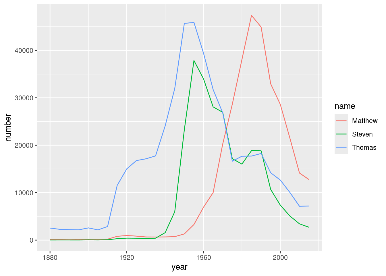
babynames %>%
  group_by(year) %>%
  mutate(year_total = sum(number)) %>%
  ungroup() %>%
  mutate(fraction = number / year_total) %>%
  group_by(name) %>%
  slice_max(fraction, n = 1)
## # A tibble: 48,040 × 5
## # Groups: name [48,040]
## year name number year_total fraction
## <dbl> <chr> <int> <int> <dbl>
## 1 2015 Aaban 15 3648781 0.00000411
## 2 2015 Aadam 22 3648781 0.00000603
## 3 2010 Aadan 11 3672066 0.00000300
## 4 2015 Aadarsh 15 3648781 0.00000411
## 5 2010 Aaden 450 3672066 0.000123
## 6 2015 Aadhav 31 3648781 0.00000850
## 7 2015 Aadhavan 5 3648781 0.00000137
## 8 2015 Aadhya 265 3648781 0.0000726
## 9 2010 Aadi 54 3672066 0.0000147
## 10 2005 Aadil 20 3828460 0.00000522
## # ℹ 48,030 more rowsbabynames %>%
group_by(name) %>%
mutate(name_total = sum(number), name_max = max(number)) %>%
ungroup() %>%
mutate(fraction_max = number/name_max)## # A tibble: 332,595 × 6
## year name number name_total name_max fraction_max
## <dbl> <chr> <int> <int> <int> <dbl>
## 1 1880 Aaron 102 114739 14635 0.00697
## 2 1880 Ab 5 77 31 0.161
## 3 1880 Abbie 71 4330 445 0.160
## 4 1880 Abbott 5 217 51 0.0980
## 5 1880 Abby 6 11272 1753 0.00342
## 6 1880 Abe 50 1832 271 0.185
## 7 1880 Abel 9 10565 3245 0.00277
## 8 1880 Abigail 12 72600 15762 0.000761
## 9 1880 Abner 27 1552 199 0.136
## 10 1880 Abraham 81 17882 2449 0.0331
## # ℹ 332,585 more rowsnames_normalized <- babynames %>%
group_by(name) %>%
mutate(name_total = sum(number),
name_max = max(number)) %>%
ungroup() %>%
mutate(fraction_max = number / name_max)names_filtered <- names_normalized %>%
filter(name %in% c("Steven", "Thomas", "Matthew"))
ggplot(names_filtered, aes(year, fraction_max, color = name))+
geom_line()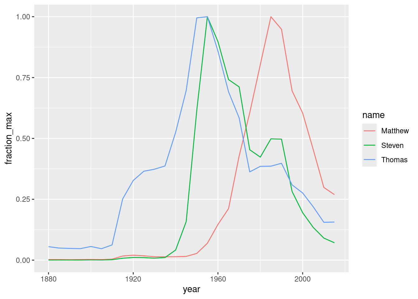
babynames_fraction <- babynames %>%
  group_by(year) %>%
  mutate(year_total = sum(number)) %>%
  ungroup() %>%
  mutate(fraction = number / year_total)
babynames_fraction %>%
arrange(name, year) %>%
group_by(name) %>%
mutate(ratio = fraction / lag(fraction))## # A tibble: 332,595 × 6
## # Groups: name [48,040]
## year name number year_total fraction ratio
## <dbl> <chr> <int> <int> <dbl> <dbl>
## 1 2010 Aaban 9 3672066 0.00000245 NA
## 2 2015 Aaban 15 3648781 0.00000411 1.68
## 3 1995 Aadam 6 3652750 0.00000164 NA
## 4 2000 Aadam 6 3767293 0.00000159 0.970
## 5 2005 Aadam 6 3828460 0.00000157 0.984
## 6 2010 Aadam 7 3672066 0.00000191 1.22
## 7 2015 Aadam 22 3648781 0.00000603 3.16
## 8 2010 Aadan 11 3672066 0.00000300 NA
## 9 2015 Aadan 10 3648781 0.00000274 0.915
## 10 2000 Aadarsh 5 3767293 0.00000133 NA
## # ℹ 332,585 more rowsbabynames_ratios_filtered <- babynames_fraction %>%
arrange(name, year) %>%
group_by(name) %>%
mutate(ratio = fraction / lag(fraction)) %>%
filter(fraction >= 0.00001)babynames_ratios_filtered %>%
group_by(name) %>%
slice_max(ratio) %>%
arrange(desc(ratio)) %>%
filter(fraction >= 0.001)## # A tibble: 291 × 6
## # Groups: name [291]
## year name number year_total fraction ratio
## <dbl> <chr> <int> <int> <dbl> <dbl>
## 1 1960 Tammy 14365 4152075 0.00346 70.1
## 2 2005 Nevaeh 4610 3828460 0.00120 45.8
## 3 1940 Brenda 5460 2301630 0.00237 37.5
## 4 1885 Grover 774 240822 0.00321 36.0
## 5 1945 Cheryl 8170 2652029 0.00308 24.9
## 6 1955 Lori 4980 4012691 0.00124 23.2
## 7 2010 Khloe 5411 3672066 0.00147 23.2
## 8 1950 Debra 6189 3502592 0.00177 22.6
## 9 2010 Bentley 4001 3672066 0.00109 22.4
## 10 1935 Marlene 4840 2088487 0.00232 16.8
## # ℹ 281 more rows