6 Joining Data with dplyr
https://learn.datacamp.com/courses/joining-data-with-dplyr
Main functions and concepts covered in this BP chapter:
inner_joinleft_joinright_joinreplace_na()is.na()full_joinsemi_joinanti_joinbind_rows
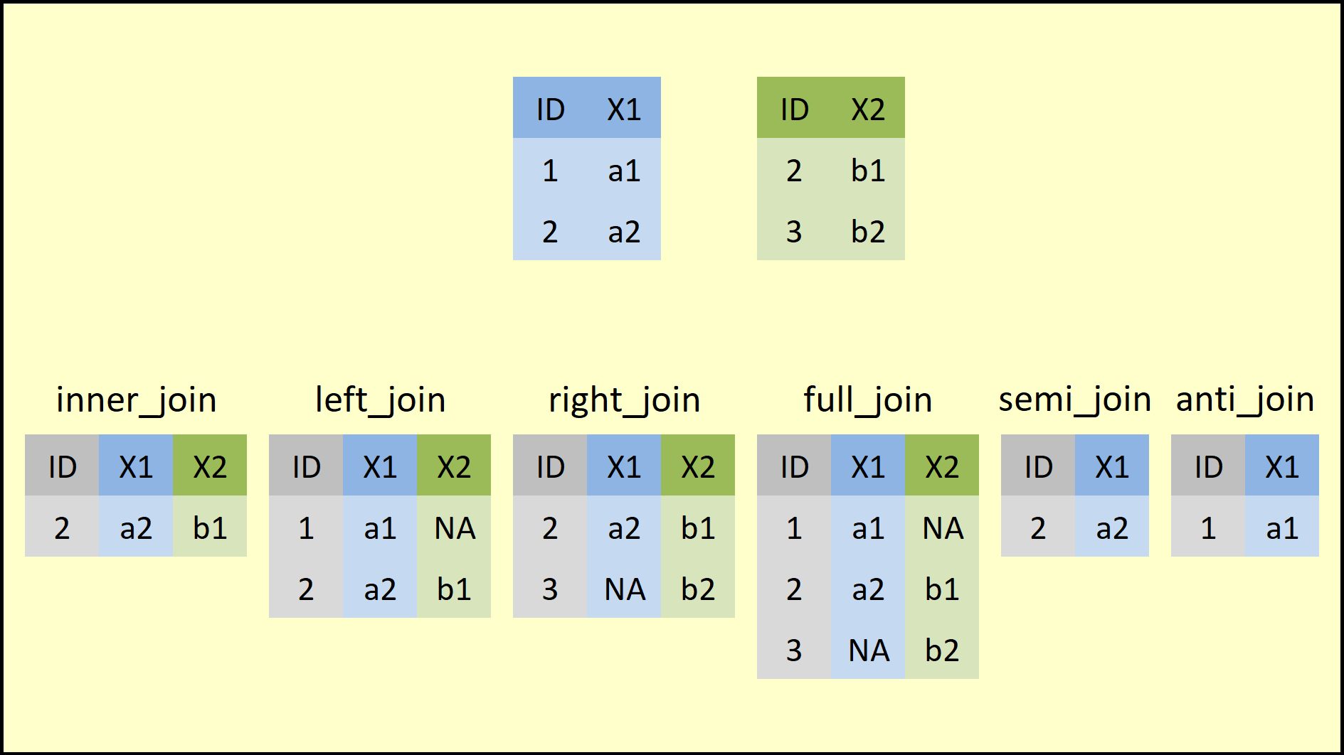
source: https://statisticsglobe.com/r-dplyr-join-inner-left-right-full-semi-anti
Packages used in this chapter:
## Load all packages used in this chapter
library(tidyverse) #includes dplyr, ggplot2, and other common packages
## ── Attaching core tidyverse packages ──────────────────────── tidyverse 2.0.0 ──
## ✔ dplyr 1.1.4 ✔ readr 2.1.6
## ✔ forcats 1.0.1 ✔ stringr 1.6.0
## ✔ ggplot2 4.0.1 ✔ tibble 3.3.0
## ✔ lubridate 1.9.4 ✔ tidyr 1.3.1
## ✔ purrr 1.2.0
## ── Conflicts ────────────────────────────────────────── tidyverse_conflicts() ──
## ✖ dplyr::filter() masks stats::filter()
## ✖ dplyr::lag() masks stats::lag()
## ℹ Use the conflicted package (<http://conflicted.r-lib.org/>) to force all conflicts to become errorsDatasets used in this chapter:
## Load datasets used in this chapter
parts <- read_rds("data/parts.rds")
part_categories <- read_rds("data/part_categories.rds")
inventory_parts <- read_rds("data/inventory_parts.rds")
inventories <- read_rds("data/inventories.rds")
sets <- read_rds("data/sets.rds")
colors <- read_rds("data/colors.rds")
themes <- read_rds("data/themes.rds")
questions <- read_rds("data/questions.rds")
question_tags <- read_rds("data/question_tags.rds")
tags <- read_rds("data/tags.rds")
answers <- read_rds("data/answers.rds")
Tip: one of the common mistakes that leads to people getting stuck in the by argument, mixing up by=c("var1"="var2") versus by=c("var1", "var2")
Note: In some exercises they have you replace NAs with 0. This is correct in these particular cases, but this is not always correct. It’s only correct if NA actually represents 0 (which it does in these exercises). (For example, if we had a dataset on people that asked how many cigarettes smoked per day and it was NA for some observations, we couldn’t assume NA means 0 because it might actually be 40 but they just didn’t answer that question.)
6.1 Joining Tables
The inner_join is the key to bring tables together. To use it, you need to provide the two tables that must be joined and the columns on which they should be joined. This returns the columns shared by both tables.
parts %>%
  inner_join(part_categories, by = c("part_cat_id" = "id"), suffix = c("_part", "_category"))
## # A tibble: 17,501 × 4
## part_num name_part part_cat_id name_category
## <chr> <chr> <dbl> <chr>
## 1 0901 Baseplate 16 x 30 with Set 080 Yellow H… 1 Baseplates
## 2 0902 Baseplate 16 x 24 with Set 080 Small Wh… 1 Baseplates
## 3 0903 Baseplate 16 x 24 with Set 080 Red Hous… 1 Baseplates
## 4 0904 Baseplate 16 x 24 with Set 080 Large Wh… 1 Baseplates
## 5 1 Homemaker Bookcase 2 x 4 x 4 7 Containers
## 6 10016414 Sticker Sheet #1 for 41055-1 58 Stickers
## 7 10026stk01 Sticker for Set 10026 - (44942/4184185) 58 Stickers
## 8 10039 Pullback Motor 8 x 4 x 2/3 44 Mechanical
## 9 10048 Minifig Hair Tousled 65 Minifig Head…
## 10 10049 Minifig Shield Broad with Spiked Bottom… 27 Minifig Acce…
## # ℹ 17,491 more rowsOften times, some of the things you care about may be a few tables away (we’ll get to that later in the course).Let’s join these two tables together to observe how joining parts with inventory_parts increases the size of your table because of the one-to-many relationship that exists between these two tables.
## # A tibble: 258,958 × 6
##    part_num name                      part_cat_id inventory_id color_id quantity
##    <chr>    <chr>                           <dbl>        <dbl>    <dbl>    <dbl>
##  1 0901     Baseplate 16 x 30 with S…           1         1973        2        1
##  2 0902     Baseplate 16 x 24 with S…           1         1973        2        1
##  3 0903     Baseplate 16 x 24 with S…           1         1973        2        1
##  4 0904     Baseplate 16 x 24 with S…           1         1973        2        1
##  5 1        Homemaker Bookcase 2 x 4…           7          508       15        1
##  6 1        Homemaker Bookcase 2 x 4…           7         1158       15        2
##  7 1        Homemaker Bookcase 2 x 4…           7         6590       15        2
##  8 1        Homemaker Bookcase 2 x 4…           7         9679       15        2
##  9 1        Homemaker Bookcase 2 x 4…           7        12256        1        2
## 10 1        Homemaker Bookcase 2 x 4…           7        13356       15        1
## # ℹ 258,948 more rows
An inner_join works the same way with either table in either position. The table that is specified first is arbitrary, since you will end up with the same information in the resulting table either way.
## # A tibble: 258,958 × 6
##    inventory_id part_num             color_id quantity name          part_cat_id
##           <dbl> <chr>                   <dbl>    <dbl> <chr>               <dbl>
##  1           21 3009                        7       50 Brick 1 x 6            11
##  2           25 21019c00pat004pr1033       15        1 Legs and Hip…          61
##  3           25 24629pr0002                78        1 Minifig Head…          59
##  4           25 24634pr0001                 5        1 Headwear Acc…          27
##  5           25 24782pr0001                 5        1 Minifig Hipw…          27
##  6           25 88646                       0        1 Tile Special…          15
##  7           25 973pr3314c01                5        1 Torso with 1…          60
##  8           26 14226c11                    0        3 String with …          31
##  9           26 2340px2                    15        1 Tail 4 x 1 x…          35
## 10           26 2340px3                    15        1 Tail 4 x 1 x…          35
## # ℹ 258,948 more rows
You can string together multiple joins with inner_join and the pipe (%>%), both with which you are already very familiar!
We’ll now connect sets, a table that tells us about each LEGO kit, with inventories, a table that tells us the specific version of a given set, and finally to inventory_parts, a table which tells us how many of each part is available in each LEGO kit.
So if you were building a Batman LEGO set, sets would tell you the name of the set, inventories would give you IDs for each of the versions of the set, and inventory_parts would tell you how many of each part would be in each version.
sets %>%
  inner_join(inventories, by = "set_num") %>%
  inner_join(inventory_parts, by = c("id" = "inventory_id"))
## # A tibble: 258,958 × 9
## set_num name year theme_id id version part_num color_id quantity
## <chr> <chr> <dbl> <dbl> <dbl> <dbl> <chr> <dbl> <dbl>
## 1 700.3-1 Medium Gift … 1949 365 24197 1 bdoor01 2 2
## 2 700.3-1 Medium Gift … 1949 365 24197 1 bdoor01 15 1
## 3 700.3-1 Medium Gift … 1949 365 24197 1 bdoor01 4 1
## 4 700.3-1 Medium Gift … 1949 365 24197 1 bslot02 15 6
## 5 700.3-1 Medium Gift … 1949 365 24197 1 bslot02 2 6
## 6 700.3-1 Medium Gift … 1949 365 24197 1 bslot02 4 6
## 7 700.3-1 Medium Gift … 1949 365 24197 1 bslot02 1 6
## 8 700.3-1 Medium Gift … 1949 365 24197 1 bslot02 14 6
## 9 700.3-1 Medium Gift … 1949 365 24197 1 bslot02a 15 6
## 10 700.3-1 Medium Gift … 1949 365 24197 1 bslot02a 2 6
## # ℹ 258,948 more rowsNow let’s join an additional table, colors, which will tell us the color of each part in each set, so that we can answer the question, “what is the most common color of a LEGO piece?”
sets %>%
  inner_join(inventories, by = "set_num") %>%
  inner_join(inventory_parts, by = c("id" = "inventory_id")) %>%
  inner_join(colors, by = c("color_id" = "id"), suffix = c("_set", "_color")) %>%
  count(name_color, sort = TRUE)
## # A tibble: 134 × 2
## name_color n
## <chr> <int>
## 1 Black 48068
## 2 White 30105
## 3 Light Bluish Gray 26024
## 4 Red 21602
## 5 Dark Bluish Gray 19948
## 6 Yellow 17088
## 7 Blue 12980
## 8 Light Gray 8632
## 9 Reddish Brown 6960
## 10 Tan 6664
## # ℹ 124 more rows6.2 Left and Right Joins
We need this to work with what they give us. You can run it at the start of this section.
inventory_parts_joined <- sets %>%
      inner_join(inventories, by = "set_num") %>%
      inner_join(inventory_parts, by = c("id" = "inventory_id")) %>%
      inner_join(colors, by = c("color_id" = "id"), suffix = c("_set", "_color")) %>%
      select(set_num, part_num, color_id, quantity)
6.2.1 left_join
left_join keeps all variables in the first table.
millennium_falcon <- inventory_parts_joined %>%
  filter(set_num == "7965-1")
star_destroyer <- inventory_parts_joined %>%
  filter(set_num == "75190-1")
millennium_falcon %>%
left_join(star_destroyer, by = c("part_num", "color_id"), suffix = c("_falcon", "_star_destroyer"))## # A tibble: 263 × 6
## set_num_falcon part_num color_id quantity_falcon set_num_star_destroyer
## <chr> <chr> <dbl> <dbl> <chr>
## 1 7965-1 12825 72 3 <NA>
## 2 7965-1 2412b 72 20 75190-1
## 3 7965-1 2412b 320 2 <NA>
## 4 7965-1 2419 71 1 <NA>
## 5 7965-1 2420 0 4 75190-1
## 6 7965-1 2420 71 1 <NA>
## 7 7965-1 2420 71 7 <NA>
## 8 7965-1 2431 72 2 <NA>
## 9 7965-1 2431 0 1 75190-1
## 10 7965-1 2431 19 2 <NA>
## # ℹ 253 more rows
## # ℹ 1 more variable: quantity_star_destroyer <dbl>In the videos and the last exercise, you joined two sets based on their part and color. What if you joined the datasets by color alone?
millennium_falcon <- inventory_parts_joined %>%
  filter(set_num == "7965-1")
star_destroyer <- inventory_parts_joined %>%
  filter(set_num == "75190-1")
millennium_falcon_colors <- millennium_falcon %>%
group_by(color_id) %>%
summarize(total_quantity = sum(quantity))
star_destroyer_colors <- star_destroyer %>%
group_by(color_id) %>%
summarize(total_quantity = sum(quantity))
millennium_falcon_colors %>%
left_join(star_destroyer_colors, by = "color_id", suffix = c("_falcon", "_star_destroyer"))## # A tibble: 21 × 3
## color_id total_quantity_falcon total_quantity_star_destroyer
## <dbl> <dbl> <dbl>
## 1 0 201 336
## 2 1 15 23
## 3 4 17 53
## 4 14 3 4
## 5 15 15 17
## 6 19 95 12
## 7 28 3 16
## 8 33 5 NA
## 9 36 1 14
## 10 41 6 15
## # ℹ 11 more rowsLeft joins are really great for testing your assumptions about a data set and ensuring your data has integrity.
inventory_version_1 <- inventories %>%
  filter(version == 1)

sets %>%
  left_join(inventory_version_1,by = "set_num" ) %>%
  filter(is.na(version))
## # A tibble: 1 × 6
## set_num name year theme_id id version
## <chr> <chr> <dbl> <dbl> <dbl> <dbl>
## 1 40198-1 Ludo game 2018 598 NA NA6.2.2 right_join
right_join returns all observations in the second table and returning matching observations in the first.
Sometimes you’ll want to do some processing before you do a join, and prioritize keeping the second (right) table’s rows instead. In this case, a right join is for you.
parts %>%
  count(part_cat_id) %>%
  right_join(part_categories, by = c("part_cat_id" = "id")) %>%
  filter(is.na(n))
## # A tibble: 1 × 3
## part_cat_id n name
## <dbl> <int> <chr>
## 1 66 NA ModulexIn both left and right joins, there is the opportunity for there to be NA values in the resulting table. Fortunately, the replace_na function can turn those NAs into meaningful values.
parts %>%
  count(part_cat_id) %>%
  right_join(part_categories, by = c("part_cat_id" = "id")) %>%
  filter(is.na(n)) %>%
  replace_na(list(n = 0))
## # A tibble: 1 × 3
## part_cat_id n name
## <dbl> <int> <chr>
## 1 66 0 ModulexTables can be joined to themselves!
In the themes table, which is available for you to inspect in the console, you’ll notice there is both an id column and a parent_id column. Keeping that in mind, you can join the themes table to itself to determine the parent-child relationships that exist for different themes.
themes %>%
  # Inner join the themes table
  inner_join(themes,by = c("id"= "parent_id"), suffix = c("_parent", "_child")) %>%
  # Filter for the "Harry Potter" parent name
  filter(name_parent == "Harry Potter")
## # A tibble: 6 × 5
## id name_parent parent_id id_child name_child
## <dbl> <chr> <dbl> <dbl> <chr>
## 1 246 Harry Potter NA 247 Chamber of Secrets
## 2 246 Harry Potter NA 248 Goblet of Fire
## 3 246 Harry Potter NA 249 Order of the Phoenix
## 4 246 Harry Potter NA 250 Prisoner of Azkaban
## 5 246 Harry Potter NA 251 Sorcerer's Stone
## 6 246 Harry Potter NA 667 Fantastic BeastsWe can go a step further than looking at themes and their children. Some themes actually have grandchildren: their children’s children.
themes %>%
  inner_join(themes, by = c("id" = "parent_id"), suffix = c("_parent", "_child")) %>%
  inner_join(themes, by = c("id_child" = "parent_id"), suffix = c("_parent", "_grandchild"))
## # A tibble: 158 × 7
## id_parent name_parent parent_id id_child name_child id_grandchild name
## <dbl> <chr> <dbl> <dbl> <chr> <dbl> <chr>
## 1 1 Technic NA 5 Model 6 Airport
## 2 1 Technic NA 5 Model 7 Constructi…
## 3 1 Technic NA 5 Model 8 Farm
## 4 1 Technic NA 5 Model 9 Fire
## 5 1 Technic NA 5 Model 10 Harbor
## 6 1 Technic NA 5 Model 11 Off-Road
## 7 1 Technic NA 5 Model 12 Race
## 8 1 Technic NA 5 Model 13 Riding Cyc…
## 9 1 Technic NA 5 Model 14 Robot
## 10 1 Technic NA 5 Model 15 Traffic
## # ℹ 148 more rowsSome themes might not have any children at all, which means they won’t be included in the inner join. As you’ve learned in this chapter, you can identify those with a left_join and a filter().
themes %>%
  # Left join the themes table to its own children
  left_join(themes, by = c("id" = "parent_id"), suffix = c("_parent", "_child")) %>%
  # Filter for themes that have no child themes
  filter(is.na(name_child))
## # A tibble: 586 × 5
## id name_parent parent_id id_child name_child
## <dbl> <chr> <dbl> <dbl> <chr>
## 1 2 Arctic Technic 1 NA <NA>
## 2 3 Competition 1 NA <NA>
## 3 4 Expert Builder 1 NA <NA>
## 4 6 Airport 5 NA <NA>
## 5 7 Construction 5 NA <NA>
## 6 8 Farm 5 NA <NA>
## 7 9 Fire 5 NA <NA>
## 8 10 Harbor 5 NA <NA>
## 9 11 Off-Road 5 NA <NA>
## 10 12 Race 5 NA <NA>
## # ℹ 576 more rows6.3 Full, Semi, and Anti Joins
6.3.1 full_join
Full joins return all columns in both tables. First, you’ll need to join in the themes. Recall that doing so requires going through the sets first. You’ll use the inventory_parts_joined table from the video.
inventory_parts_joined <- inventories %>%
  inner_join(inventory_parts, by = c("id" = "inventory_id")) %>%
  arrange(desc(quantity)) %>%
  select(-id, -version)

inventory_sets_themes <-inventory_parts_joined %>%
  inner_join(sets, by = "set_num") %>%
  inner_join(themes, by = c("theme_id" = "id"), suffix = c("_set", "_theme"))
Previously, you combined tables to compare themes. Before doing this comparison, you’ll want to aggregate the data to learn more about the pieces that are a part of each theme, as well as the colors of those pieces.
batman <- inventory_sets_themes %>%
  filter(name_theme == "Batman")

star_wars <- inventory_sets_themes %>%
  filter(name_theme == "Star Wars")

batman_parts <- batman %>%
  count(part_num,color_id, wt = quantity)

star_wars_parts <- star_wars %>%
  count(part_num, color_id, wt = quantity)
Now that you’ve got separate tables for the pieces in the batman and star_wars themes, you’ll want to be able to combine them to see any similarities or differences between the two themes.
parts_joined <- batman_parts %>%
  full_join(star_wars_parts,by = c("part_num", "color_id"),suffix = c("_batman", "_star_wars")) %>%
  replace_na(list(n_batman = 0,
                  n_star_wars = 0))
The table you created in the last exercise includes the part number of each piece, the color id, and the number of each piece in the Star Wars and Batman themes. However, we have more information about each of these parts that we can gain by combining this table with some of the information we have in other tables.
parts_joined %>%
  arrange(desc(n_star_wars)) %>%
  inner_join(colors, by = c("color_id" = "id")) %>%
  inner_join(parts, by = "part_num", suffix = c("_color", "_part"))
## # A tibble: 3,628 × 8
## part_num color_id n_batman n_star_wars name_color rgb name_part part_cat_id
## <chr> <dbl> <dbl> <dbl> <chr> <chr> <chr> <dbl>
## 1 2780 0 104 392 Black #051… Technic … 53
## 2 32062 0 1 141 Black #051… Technic … 46
## 3 4274 1 56 118 Blue #005… Technic … 53
## 4 6141 36 11 117 Trans-Red #C91… Plate Ro… 21
## 5 3023 71 10 106 Light Blu… #A0A… Plate 1 … 14
## 6 6558 1 30 106 Blue #005… Technic … 53
## 7 43093 1 44 99 Blue #005… Technic … 53
## 8 3022 72 14 95 Dark Blui… #6C6… Plate 2 … 14
## 9 2357 19 0 84 Tan #E4C… Brick 2 … 11
## 10 6141 179 90 81 Flat Silv… #898… Plate Ro… 21
## # ℹ 3,618 more rows6.3.2 semi_join and anti_join
In the videos, you learned how to filter using the semi- and anti join verbs to answer questions you have about your data. Let’s focus on the batwing dataset, and use our skills to determine which parts are in both the batwing and batmobile sets, and which sets are in one, but not the other. While answering these questions, we’ll also be determining whether or not the parts we’re looking at in both sets also have the same color in common.
semi_join returns all columns also found in the joining table, while anti_join returns all columns not included in the second table.
batmobile <- inventory_parts_joined %>%
  filter(set_num == "7784-1") %>%
  select(-set_num)

batwing <- inventory_parts_joined %>%
  filter(set_num == "70916-1") %>%
select(-set_num)## # A tibble: 126 × 3
## part_num color_id quantity
## <chr> <dbl> <dbl>
## 1 3023 0 22
## 2 3024 0 22
## 3 3623 0 20
## 4 2780 0 17
## 5 3666 0 16
## 6 3710 0 14
## 7 6141 4 12
## 8 2412b 71 10
## 9 6141 72 10
## 10 6558 1 9
## # ℹ 116 more rows## # A tibble: 183 × 3
## part_num color_id quantity
## <chr> <dbl> <dbl>
## 1 11477 0 18
## 2 99207 71 18
## 3 22385 0 14
## 4 99563 0 13
## 5 10247 72 12
## 6 2877 72 12
## 7 61409 72 12
## 8 11153 0 10
## 9 98138 46 10
## 10 2419 72 9
## # ℹ 173 more rowsBesides comparing two sets directly, you could also use a filtering join like semi_join to find out which colors ever appear in any inventory part. Some of the colors could be optional, meaning they aren’t included in any sets.
## # A tibble: 134 × 3
##       id name           rgb
##    <dbl> <chr>          <chr>
##  1    -1 [Unknown]      #0033B2
##  2     0 Black          #05131D
##  3     1 Blue           #0055BF
##  4     2 Green          #237841
##  5     3 Dark Turquoise #008F9B
##  6     4 Red            #C91A09
##  7     5 Dark Pink      #C870A0
##  8     6 Brown          #583927
##  9     7 Light Gray     #9BA19D
## 10     8 Dark Gray      #6D6E5C
## # ℹ 124 more rows
version_1_inventories <- inventories %>%
filter(version == 1)
sets %>%
anti_join(version_1_inventories, by = "set_num")## # A tibble: 1 × 4
## set_num name year theme_id
## <chr> <chr> <dbl> <dbl>
## 1 40198-1 Ludo game 2018 5986.3.3 Visualizing set differences
To compare two individual sets, and the kinds of LEGO pieces that comprise them, we’ll need to aggregate the data into separate themes. Additionally, as we saw in the video, we’ll want to add a column so that we can understand the fractions of specific pieces that are part of each set, rather than looking at the numbers of pieces alone.
inventory_parts_themes <- inventories %>%
  inner_join(inventory_parts, by = c("id" = "inventory_id")) %>%
  arrange(desc(quantity)) %>%
  select(-id, -version) %>%
  inner_join(sets, by = "set_num") %>%
  inner_join(themes, by = c("theme_id" = "id"), suffix = c("_set", "_theme"))

inventory_parts_themes
## # A tibble: 258,958 × 9
## set_num part_num color_id quantity name_set year theme_id name_theme
## <chr> <chr> <dbl> <dbl> <chr> <dbl> <dbl> <chr>
## 1 40179-1 3024 72 900 Personalised M… 2016 277 Mosaic
## 2 40179-1 3024 15 900 Personalised M… 2016 277 Mosaic
## 3 40179-1 3024 0 900 Personalised M… 2016 277 Mosaic
## 4 40179-1 3024 71 900 Personalised M… 2016 277 Mosaic
## 5 40179-1 3024 14 900 Personalised M… 2016 277 Mosaic
## 6 k34434-1 3024 15 810 Lego Mosaic Ti… 2003 277 Mosaic
## 7 21010-1 3023 320 771 Robie House 2011 252 Architect…
## 8 k34431-1 3024 0 720 Lego Mosaic Cat 2003 277 Mosaic
## 9 42083-1 2780 0 684 Bugatti Chiron 2018 5 Model
## 10 k34434-1 3024 0 540 Lego Mosaic Ti… 2003 277 Mosaic
## # ℹ 258,948 more rows
## # ℹ 1 more variable: parent_id <dbl>batman_colors <- inventory_parts_themes %>%
filter(name_theme == "Batman") %>%
group_by(color_id) %>%
summarize(total = sum(quantity)) %>%
mutate(fraction = total/sum(total))
batman_colors## # A tibble: 57 × 3
## color_id total fraction
## <dbl> <dbl> <dbl>
## 1 0 2807 0.296
## 2 1 243 0.0256
## 3 2 158 0.0167
## 4 4 529 0.0558
## 5 5 1 0.000105
## 6 10 13 0.00137
## 7 14 426 0.0449
## 8 15 404 0.0426
## 9 19 142 0.0150
## 10 25 36 0.00380
## # ℹ 47 more rowsstar_wars_colors <- inventory_parts_themes %>%
filter(name_theme == "Star Wars") %>%
group_by(color_id) %>%
summarize(total = sum(quantity)) %>%
mutate(fraction = total/sum(total))
star_wars_colors## # A tibble: 52 × 3
## color_id total fraction
## <dbl> <dbl> <dbl>
## 1 0 3258 0.207
## 2 1 410 0.0261
## 3 2 36 0.00229
## 4 3 25 0.00159
## 5 4 434 0.0276
## 6 6 40 0.00254
## 7 7 209 0.0133
## 8 8 51 0.00324
## 9 10 6 0.000382
## 10 14 207 0.0132
## # ℹ 42 more rowsPrior to visualizing the data, you’ll want to combine these tables to be able to directly compare the themes’ colors.
colors_joined <- batman_colors %>%
  full_join(star_wars_colors, by = "color_id", suffix = c("_batman", "_star_wars")) %>%
  replace_na(list(total_batman = 0,
  total_star_wars = 0)) %>%
  inner_join(colors, by = c("color_id" = "id")) %>%
  mutate(difference = fraction_batman - fraction_star_wars,
         total = total_batman + total_star_wars) %>%
  filter(total >= 200)
# For some reason I got one color with a difference of NA...
# you don't have to drop it, but you avoid an error if you do.
# Even better is figuring out how to avoid the NA in the first place...
# You also need to arrange the data by difference (that's how it is in the graph)
colors_joined <- colors_joined %>% arrange(difference) %>% filter(!is.na(difference))
# These two lines get the color names to display in order of difference.
# There are other ways (they mention the "forcats" package in the video),
# but like many things, I googled it and I found a solution tat I adapted to this and it worked
colors_joined$name <- as.character(colors_joined$name)
colors_joined$name <- factor(colors_joined$name, levels=colors_joined$name)
# Create the color palette itself, which is just the colors and their names
color_palette_df <- colors %>%
semi_join(colors_joined, by = c("id" = "color_id")) %>%
select(-id)
color_palette <- color_palette_df$rgb
names(color_palette) <- color_palette_df$nameIn the last exercise, you created colors_joined. Now you’ll create a bar plot with one bar for each color (name), showing the difference in fractions.
ggplot(colors_joined, aes(name, difference, fill = name)) +
  geom_col() +
  coord_flip() +
  scale_fill_manual(values = color_palette, guide = "none") +
  labs(y = "Difference: Batman - Star Wars")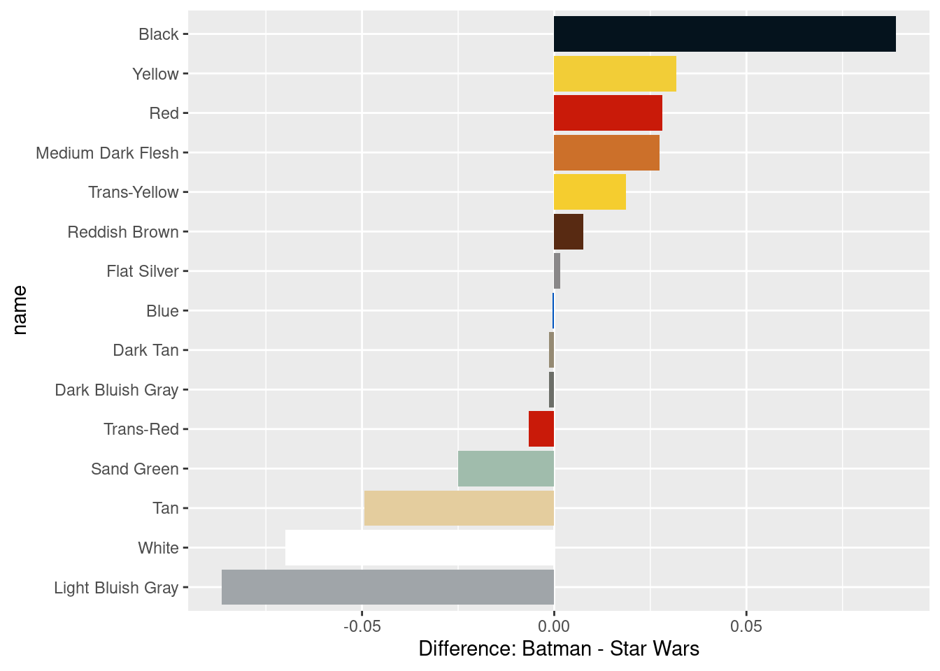
6.4 Case Study: Joins on Stack Overflow Data
Three of the Stack Overflow survey datasets are questions, question_tags, and tags:
questions: an ID and the score, or how many times the question has been upvoted; the data only includes R-based questionsquestion_tags: a tag ID for each question and the question’s idtags: a tag id and the tag’s name, which can be used to identify the subject of each question, such as ggplot2 or dplyr
questions_with_tags <- questions %>%
  left_join(question_tags, by = c("id" = "question_id")) %>%
  left_join(tags, by = c("tag_id" = "id")) %>%
  replace_na(list(tag_name = "only-r"))

questions_with_tags
## # A tibble: 545,694 × 5
## id creation_date score tag_id tag_name
## <int> <date> <int> <dbl> <chr>
## 1 22557677 2014-03-21 1 18 regex
## 2 22557677 2014-03-21 1 139 string
## 3 22557677 2014-03-21 1 16088 time-complexity
## 4 22557677 2014-03-21 1 1672 backreference
## 5 22557707 2014-03-21 2 NA only-r
## 6 22558084 2014-03-21 2 6419 time-series
## 7 22558084 2014-03-21 2 92764 panel-data
## 8 22558395 2014-03-21 2 5569 function
## 9 22558395 2014-03-21 2 134 sorting
## 10 22558395 2014-03-21 2 9412 vectorization
## # ℹ 545,684 more rowsquestions_with_tags %>%
group_by(tag_name) %>%
summarize(score = mean(score),
num_questions = n()) %>%
arrange(desc(num_questions))## # A tibble: 7,841 × 3
## tag_name score num_questions
## <chr> <dbl> <int>
## 1 only-r 1.26 48541
## 2 ggplot2 2.61 28228
## 3 dataframe 2.31 18874
## 4 shiny 1.45 14219
## 5 dplyr 1.95 14039
## 6 plot 2.24 11315
## 7 data.table 2.97 8809
## 8 matrix 1.66 6205
## 9 loops 0.743 5149
## 10 regex 2 4912
## # ℹ 7,831 more rows## # A tibble: 40,459 × 2
## id tag_name
## <dbl> <chr>
## 1 124399 laravel-dusk
## 2 124402 spring-cloud-vault-config
## 3 124404 spring-vault
## 4 124405 apache-bahir
## 5 124407 astc
## 6 124408 simulacrum
## 7 124410 angulartics2
## 8 124411 django-rest-viewsets
## 9 124414 react-native-lightbox
## 10 124417 java-module
## # ℹ 40,449 more rowsNow we’ll join together questions with answers so we can measure the time between questions and answers.
questions %>%
  inner_join(answers, by = c("id" = "question_id"), suffix = c("_question", "_answer")) %>%
  mutate(gap = as.integer(creation_date_answer - creation_date_question))
## # A tibble: 380,643 × 7
## id creation_date_question score_question id_answer creation_date_answer
## <int> <date> <int> <int> <date>
## 1 22557677 2014-03-21 1 22560670 2014-03-21
## 2 22557707 2014-03-21 2 22558516 2014-03-21
## 3 22557707 2014-03-21 2 22558726 2014-03-21
## 4 22558084 2014-03-21 2 22558085 2014-03-21
## 5 22558084 2014-03-21 2 22606545 2014-03-24
## 6 22558084 2014-03-21 2 22610396 2014-03-24
## 7 22558084 2014-03-21 2 34374729 2015-12-19
## 8 22558395 2014-03-21 2 22559327 2014-03-21
## 9 22558395 2014-03-21 2 22560102 2014-03-21
## 10 22558395 2014-03-21 2 22560288 2014-03-21
## # ℹ 380,633 more rows
## # ℹ 2 more variables: score_answer <int>, gap <int>We can also determine how many questions actually yield answers. If we count the number of answers for each question, we can then join the answers counts with the questions table.
answer_counts <- answers %>%
  count(question_id, sort = TRUE)

question_answer_counts <- questions %>%
  left_join(answer_counts, by = c("id" = "question_id")) %>%
  replace_na(list(n = 0))
Let’s build on the last exercise by adding the tags table to our previous joins. This will allow us to do a better job of identifying which R topics get the most traction on Stack Overflow.
tagged_answers <- question_answer_counts %>%
  inner_join(question_tags, by = c("id" = "question_id")) %>%
  inner_join(tags, by = c("tag_id" = "id"))
You can use this table to determine, on average, how many answers each questions gets.
tagged_answers %>%
  group_by(tag_name) %>%
  summarize(questions = n(),
            average_answers = mean(n)) %>%
  arrange(desc(questions))
## # A tibble: 7,840 × 3
## tag_name questions average_answers
## <chr> <int> <dbl>
## 1 ggplot2 28228 1.15
## 2 dataframe 18874 1.67
## 3 shiny 14219 0.921
## 4 dplyr 14039 1.55
## 5 plot 11315 1.23
## 6 data.table 8809 1.47
## 7 matrix 6205 1.45
## 8 loops 5149 1.39
## 9 regex 4912 1.91
## 10 function 4892 1.30
## # ℹ 7,830 more rowsquestions_with_tags <- questions %>%
inner_join(question_tags, by = c("id" = "question_id")) %>%
inner_join(tags, by = c("tag_id" = "id"))
questions_with_tags## # A tibble: 497,153 × 5
## id creation_date score tag_id tag_name
## <int> <date> <int> <dbl> <chr>
## 1 22557677 2014-03-21 1 18 regex
## 2 22557677 2014-03-21 1 139 string
## 3 22557677 2014-03-21 1 16088 time-complexity
## 4 22557677 2014-03-21 1 1672 backreference
## 5 22558084 2014-03-21 2 6419 time-series
## 6 22558084 2014-03-21 2 92764 panel-data
## 7 22558395 2014-03-21 2 5569 function
## 8 22558395 2014-03-21 2 134 sorting
## 9 22558395 2014-03-21 2 9412 vectorization
## 10 22558395 2014-03-21 2 18621 operator-precedence
## # ℹ 497,143 more rowsanswers_with_tags <- answers %>%
inner_join(question_tags, by = "question_id") %>%
inner_join(tags, by = c("tag_id" = "id"))## Warning in inner_join(., question_tags, by = "question_id"): Detected an unexpected many-to-many relationship between `x` and `y`.
## ℹ Row 3 of `x` matches multiple rows in `y`.
## ℹ Row 156352 of `y` matches multiple rows in `x`.
## ℹ If a many-to-many relationship is expected, set `relationship =
## "many-to-many"` to silence this warning.## # A tibble: 625,845 × 6
## id creation_date question_id score tag_id tag_name
## <int> <date> <int> <int> <dbl> <chr>
## 1 39143935 2016-08-25 39142481 0 4240 average
## 2 39143935 2016-08-25 39142481 0 5571 summary
## 3 39144014 2016-08-25 39024390 0 85748 shiny
## 4 39144014 2016-08-25 39024390 0 83308 r-markdown
## 5 39144014 2016-08-25 39024390 0 116736 htmlwidgets
## 6 39144252 2016-08-25 39096741 6 67746 rstudio
## 7 39144375 2016-08-25 39143885 5 105113 data.table
## 8 39144430 2016-08-25 39144077 0 276 variables
## 9 39144625 2016-08-25 39142728 1 46457 dataframe
## 10 39144625 2016-08-25 39142728 1 9047 subset
## # ℹ 625,835 more rowsFirst, you’ll want to combine these tables into a single table called posts_with_tags. Once the information is consolidated into a single table, you can add more information by creating a date variable using the lubridate package.
posts_with_tags <- bind_rows(questions_with_tags %>% mutate(type = "question"),
                              answers_with_tags %>% mutate(type = "answer"))

by_type_year_tag <-  posts_with_tags %>%
  mutate(year = year(creation_date)) %>%
  count(type, year, tag_name)
by_type_year_tag
## # A tibble: 58,299 × 4
## type year tag_name n
## <chr> <dbl> <chr> <int>
## 1 answer 2008 bayesian 1
## 2 answer 2008 dataframe 3
## 3 answer 2008 dirichlet 1
## 4 answer 2008 eof 1
## 5 answer 2008 file 1
## 6 answer 2008 file-io 1
## 7 answer 2008 function 7
## 8 answer 2008 global-variables 7
## 9 answer 2008 math 2
## 10 answer 2008 mathematical-optimization 1
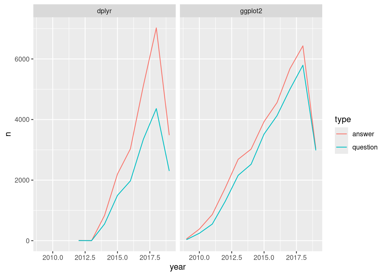
## # ℹ 58,289 more rowsIn the last exercise, you modified the posts_with_tags table to add a year column, and aggregated by type, year, and tag_name. The modified table has been preloaded for you as by_type_year_tag, and has one observation for each type (question/answer), year, and tag. Let’s create a plot to examine the information that the table contains about questions and answers for the dplyr and ggplot2 tags.
by_type_year_tag_filtered <- by_type_year_tag %>%
  filter(tag_name %in% c("dplyr", "ggplot2"))

ggplot(by_type_year_tag_filtered, aes(year, n, color = type)) +
  geom_line() +
  facet_wrap(~ tag_name)